Many relevant diagnostic signs are not performed deliberately by the examiner or by the patient at the examiner’s direction. They are observed as the patient reacts to their condition. Fortin’s finger sign, Minor’s sign, and Vanzetti’s sign are three examples of this principle.
Scientific Writing: Discriminating Good from Bad
In the earlier parts of this series we explored ways of evaluating scientific writing by considering the critical issues of study design, assignment of study and control groups, assessment of outcome, and finally, interpretation and extrapolation of results. We also looked at different study types. In this part we'll take a look at ways of reporting our results.
When a new test is developed, and this could be a laboratory test, an orthopaedic test, an electrodiagnostic test, etc., it is tested against the existing gold standard test. Two of the most commonly reported results are sensitivity and specificity. Sensitivity is a measurement of the proportion of people who actually have the disease and are correctly identified, i.e., the percentage of true positives. Conversely, the specificity of a test is a reflection of the proportion of those who do not have the disease and who are correctly identified as being disease-free by the test. These measures tell us only the proportions of people who are diseased and disease-free. Most importantly, these figures measure the discriminate ability of the test. Let's look at an example of a new test which is compared to the existing gold standard. In this study we have 1,000 individuals, of which 600 have been identified as having a disease and 400 have been identified as disease-free.

In the above example the new test has correctly identified 500 of the 600 persons who actually do have the disease (according to our gold standard). However, it has failed to identify 100 who are diseased. Thus, there are 100 false negatives. This gives the test a sensitivity of 83 percent. Also correctly identified were 350 of 400 who were classified as disease-free, while 50 were falsely identified as having the disease. This gives us a specificity of 88 percent.
Since both of these calculations are derived from separate columns (i.e., a/a+c and d/b+d) the relative proportions of diseased and disease-free individuals in the study does not affect our calculation. However, the prevalence of a disease in a given population will have a definite impact on the relative numbers of false positives and false negatives. Let's look at two examples of different prevalences (5 percent and 50 percent) and, using our earlier results of 83 percent sensitivity and 88 percent specificity, calculate the number of false negatives and false positives we can expect in the two populations.

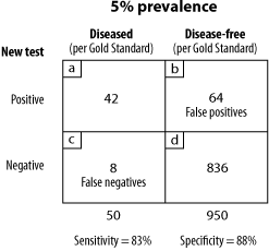
In this example we will assume that, out of 1000 people, 950 are disease-free and 50 have the disease. Working backward we can calculate that 42 will be correctly identified as diseased (.83 x 50=42) and the remaining 8 will be false negatives. And we can likewise calculate that 836 will be correctly identified as disease-free (.88x950=836) with the remaining 64 as false positives, (Fig. 2). In this case we have a 5 percent prevalence of disease in our population (50/(50+950)=.05). With a 50 percent prevalence of disease our calculations would yield the figures shown in FIG. 3.
Notice that in the lower prevalence population we actually have more false positives than true positives, illustrating an important concept in statistics. Even though sensitivity and specificity calculations are not influenced by the prevalence of a disease in a given population, the number of false positives and false negatives identified are. This may seem confusing or ambiguous at first, but in a moment it will make perfect sense. Let's look at a real example of how this can apply to research.

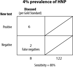
In a project designed to detect disc herniation in two populations, one with a prevalence of four percent and one with a prevalence of 25 percent, and using tools that provided 80 percent and 98 percent sensitivity, the authors of one study concluded that the more sensitive test used on the larger prevalence population would likely yield fewer false positives than using the less sensitive test on the lower prevalence population. But they were wrong (Figs. 4 and 5). And as we have seen, if a condition has a very low prevalence in a population even a very highly specific test might give us more false positives than true positives.
The predictive value of a test is a measure of the test's ability to either rule in or rule out a disease because it tells us how likely it is that someone with a positive test actually does have a disease (positive predictive value) or how likely it is that someone with a negative test actually does not have a disease (negative predictive value). We can use the same examples as we had in Figs. 2 & 3 just to save space. When we calculated sensitivity and specificity earlier, we were concerned only with the (vertical) columns of our 2 x 2 tables. Now we will calculate across rows (horizontally). Those mathematically inclined will realize that in this calculation the prevalence does become important.

Positive predictive value is calculated as a/a+b, whereas negative predictive value is equal to d/c+d. If a test has a high positive predictive value it means that a positive test strongly indicates that the patient does have the disease in question. Likewise, when the negative predictive value is high we can be fairly confident that in a patient with a negative test, no disease is present, i.e., that the likelihood of false negative is low.
Referring back to Fig. 2, the population with a five percent prevalence, we can calculate these values as follows:
Positive predictive value = a/a+b = 42/(42+64) = 40 percent
Negative predictive value = d/c+d = 836/(8+836) = 99 percent
These results are not surprising since we found that there were more false positive than true positives -- we can't place too much faith in a positive test when there's a 60 percent chance it should have been negative. Now let's look at Fig. 3, the population with a 50 percent prevalence:
Positive predictive value = a/a+b = 415/415+60 = 87 percent
Negative predictive value = d/c+d = 440/85+440 = 83 percent

It now becomes quite clear that to judge the predictive value of a test we must have a fairly good estimate of the prevalence of the disease (or condition) tested for in a given population. The lower the prevalence of the disease, the lower the positive predictive value of a test and, as we've seen, the same test with good sensitivity and specificity may be quite reliable in one population but nearly useless in another.
With an understanding of these measurements you can see how researchers can effectively stack the deck in a given project, an approach which is usually not deliberate but which can sometimes yield results that are misleading. Naturally, when we take a study population of 100 patients, 80 of which have the given disorder we intend to look for with our new test, it is quite likely that we will wind up with fairly impressive figures. However, we must ask ourselves an important question about the true prevalence of the condition in the real population of patients we are likely to see in our offices. If the prevalence is only three percent rather than 80 percent how much confidence can we put it the test? Now you can figure it out yourself if you know the sensitivity and specificity of the test and the approximate prevalence of the disorder.


